Autosum In Excel

Autosum Command 

What you do the most frequent in excel ?That is definitely the adding up numbers .The shortcut for doing the same is Autosum in excel.
.

Keyboard short cut for Autosum is     "Alt+equal sign(=)"

Case 2
What if you want to get the sum of each column  row & grand sum  in one command for the data given below

Generating List Of Sheet Names In A Workbook

Microsoft Excel doesn’t provide a direct way to generate a list of sheet names in a workbook. Here is a small macro to generate the  list of all the sheets in a workbook.

First you open a workbook which contains lot of worksheets and follow the steps

Step 1 : Insert a new worksheet where you want the worksheet names to be displayed 

Step 2  Goto –VIEW –MACROS-VIEW [Here I am using Excel 2013 so the tabs are slightly different from the version you might be using ;excel 2007 or Excel 2010 .But dont worry :D]

.

Step 3:In “Macro name” column  please write WorksheetName [This is the name of the macro] 

.

Step 4 Click On Create Button.You will Get a sceen like this

.

Step 5 Paste the following argument between  “Sub WorksheetName()”   and “End Sub”

Dim x As Integer

For x = 1 To Worksheets.Count

Cells(x, 1).Value = Worksheets(x).Name

Next x 

.

Step 6 :Close the Macro window

Now the macro is ready to run .

How to Run The Macro 

goto  “VIEW” Tab- MACROS-VIEW MACRO -RUN

Excel Shortcuts

Show All Formula

You can view all the formulas used in the worksheet by simultaneously Pressing  CTRL and ~ 

This symbol ~ usually found on the key to the left of number 1 key in the keyboard 

eg :

Inorder see the equation used in the column D ,just select the column or the entire worksheet and then press  CTRL and ~

To goback to the orginal one click CTRL ~ again

Excel Match

 Excel MATCH function searches for a value in an array and returns the relative position of that item.

Match function in excel is used to searches for the value of item in an array and returns the relative position of that Item. 

Syntax of the match function "MATCH(Value looking For , Lookup Array, Match type)

Value Looking For :- The value that you want to find in the list of data. It  be a number, text, logical value, or a cell reference .

Lookup Array :-The range of cells need to be  searched

Match type for exact match is "0".

Example:-

If we want find the position of Vinoy in the list ,we can use Match function.

It is a very useful Function in Excel.

Background-Image-for-Chart-In-Excel

How To Create A Chart With A Background Image 

Eg:-% Of Marks Obtained By Some MBC College Students with College Photo as Background 

Step 1
Arrange the data

Step 2
Select the data and create a chart

.








Step 3
Right click On chart ----Select "Format Chart Area"
Select a background Image

Step 4
Click on the chart ---Goto "Home" Tab -----Click on "Colors" and Put "Transparency" 40% Click OK

Chart is ready with a background pic

VLOOKUP 

Sometimes you may come up with situations to lookup the data in a same  work sheet or  different work sheet or sometimes even from a different work book .

The Most common lookup function is the VLOOKUP [Vertical Lookup].

Excel VLOOKUP is one of the most useful function, and unfortunately it’s also one of the least understood. Here I will explain  how to use Vlookup with some simple examples .

The given is the list of items our company sells

In this example I have mentioned  only 4 items .But in real situations you might have 1000’s of different items.

Now here is a situation where we just know only  the Item code and we want to know what is the Item name .

so in this  situation we can use Vlookup function

Steps

1 .Select Vlookup function from Lookup & Reference in "Formulas"

2. Click On VLookup function

3.Select all the Values mentioned in the Table 

      Here Lookup value is the Item Code . Which is coming in the A11 Cell 
      
     Table_Array -Is the Reference Table which we are looking for the Item .So we need to select the entire table [Table Name -List Of Items]
     
    Col_Index_num - Is the Column number in the table -array from which the matching value should be returned .Here Col_Index_num is "2" ,where the item name is given.

  Range Lookup -Is a Logical Value .For Exact match we should use FALSE or 0 And for approx match we should use TRUE or 1 

4 Click On OK 

We will get the following result 

This is a simple example for Vlookup function and in the coming blog we will see some complex situvations where we can use the Vlookup function

Combining Cells- Concatenate

In order to combine 2 or more cells we can use a function  called "CONCATENATE" .It is one of the most useful function in Excel .

Syntax: Concatenate(text1,text 2,...)

Example:

Note :For giving space between words, we should give a space in between two double quotes. 

Watch Window

You can use watch window to keep track of data in a particular cell or range of cell even when the cells are no longer in view .This is especially useful when you want to keep your eye on a specific formula or cell you use to create a formula .You can also use a watch window to keep track of particular cell's data as you work with the rest of your work sheet.


Example :-


You are running a stationary shop and  entering the stock which you are planning for the next month .After entering each item you want to know the total amount of entire stock  .Here you can use watch window on the cell where we are calculating the sum of all stock.

Here you want to keep an eye on Total stock amount [E15 cell]after each item entry  .
[E15 cell is the sum of all stock amount]


Steps


Click Formula Tab  then Click On Watch Window

Click on the particular cell we want to watch ,here it is E15 

Select the cell or Cells you want to watch .You can also type the cell reference.


Click Add 


Then a new window will come which will show you the value of that particular cell along with the formula applied in that cell.

If we enter a new item or change the value of any item we can always see the total of all stocks in "Watch Window"


Note : You can add multiple cells to the watch window 

Pivot table in excel

PIVOT TABLE

Pivot table in excel is  the most powerful and very useful feature of Microsoft Excel .It is a great tool for sorting and summarizing the data in a spreadsheet. It be used to summarize, analyze, explore and present your data in a meaningful way .

I have seen many people are not using Pivot table as they think that it is a very tough  tool to learn & use .Even i thought the same some years back .

Instead of analyzing countless spreadsheet records, a pivot table can aggregate your information and show a new perspective in a few clicks.

Example :

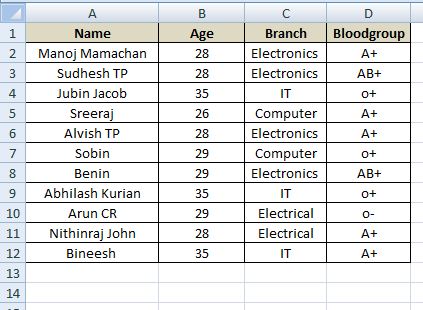
Given below are ID card details of some of my batch mates .The information provided in the ID card are:-

• Name 
• Age 
• Branch
• Blood group

Using Pivot table we can resolve so many queries we have regarding the information given in the table 

• How many students have got the same blood group and their names
• How many are in the   same age 
• Which are the different branches etc etc etc....

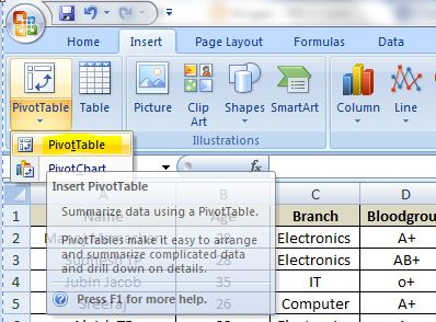
How to make Pivot Table

Goto Insert Tab-Pivot Table 

Click on  Pivot Table 

Then Select the Range of Cells 

Please select New Work Sheet 

We will Move to a new Sheet Like This 

So Pivot Table Is Ready .Now We are going to Resolve our Queries

1.How Many Students Have Got The Same Blood Group And Their Name 

You Have to Drag and Drop the concerned  Field (Blood-group & Name ) Into Raw Label  

II) How many Are In The  Same Age 

III) Different Branches ,Names & Age 

Another Presentation for the same will be 

This is Just the starting of Pivot Table .We can do filtering Additional formatting etc in our Pivot table ,That we will discuss in the next Section 

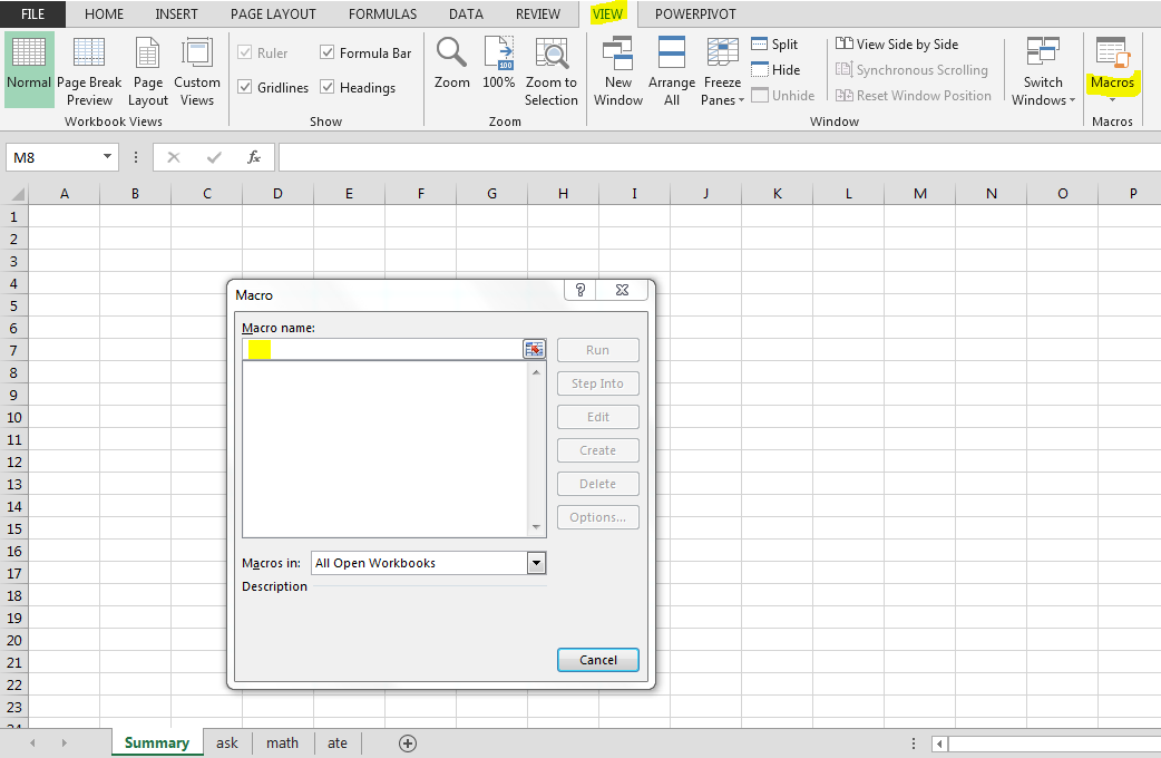
Note :You can easily change the pivot table summary formulas. Right click on pivot table and select “ summarize data by” option

How to Count Words In A Cell

Sometimes we might come into a situation that we should know what is the  the number of words in a particular  cell .

Eg: Given below are the name of 4 engineering colleges in Kerala .Here we want to know how many words are the in the name of  each college 

The formula for finding out the number of words in a cell is 

LEN(Ref Cell )-LEN(SUBSTITUTE(Ref Cell," ",""))+1

How To Insert A Line Break 

In most of the programs you have to click Enter Key to move the cursor to the next line .But in Excel  if you press enter then the cursor will jump to the next cell .But if we want not to go to the next cell ,but in the same cell & want to type something in the next line 

Then Press ALT+ENTER 

Note :While using formulas pls use char(10) instead of ALT+ENTER

Close All Worksheets Together 

If you are working with multiple worksheet and want to close all worksheet together then


Press Shift Key and Close any of the  worksheet then all the worksheets will get close together.


Note :If any of the worksheet  have not been saved, you'll get the standard prompt asking "if you want to save your workbook".